Last week, a colleague draw my attention on this new log files from the Rstudio cloud CRAN mirror, through a post from Tal Galili. This CRAN mirror is a little different, as it uses Amazon CloudFront to deliver the downloads rapidly from a server near you, wherever that is. But what’s really great about it, is the availability of those log files, that have been recording every package download since October 2012, daily! As R is primarily intended for statisticians, it didn’t take long before we start playing with the data. Below is my bit to this effort, a function to plot the world map of one’s package downloads from the Rstudio “0-Cloud” CRAN mirror. It relies on Tal Galili’s functions for downloading and formating the data. Of course, the Rstudio CRAN mirror is only 1 mirror among all the CRAN mirrors around the world, and is not representative due to its link with the Rstudio IDE. However, in research, there is quite a delay between one’s hard work (i.e. implementing a package) and the reward (i.e. publication). Encouragements such as download stats are welcomed!
pkgDNLs.worldmapcolor <- function(pkgname, rmvdupips = TRUE, date.start = Sys.Date() -
8, date.stop = Sys.Date() - 1, shp.file.repos) {
library(installr)
library(ggplot2)
library(maptools)
if (date.stop >= Sys.Date() | date.start >= Sys.Date()) {
stop("date not available yet")
}
cat("downloading the RStudio CRAN data...\n")
dnldata_folder <- download_RStudio_CRAN_data(START = date.start, END = date.stop)
cat("data downloaded!\n")
dnldata <- read_RStudio_CRAN_data(dnldata_folder)
data <- dnldata[which(dnldata$package == pkgname), ]
if (rmvdupips) {
data <- data[!duplicated(data$ip_id), ]
}
counts <- cbind.data.frame(table(data$country))
names(counts) <- c("country", "count")
# you need to download a shapefile of the world map from Natural Earth (for
# instance)
# http://www.naturalearthdata.com/http//www.naturalearthdata.com/download/110m/cultural/ne_110m_admin_0_countries.zip
# and unzip it in the 'shp.file.repos' repository
world <- readShapePoly(fn = paste(shp.file.repos, "ne_110m_admin_0_countries",
sep = "/"))
ISO_full <- as.character(world@data$iso_a2)
ISO_full[146] <- "SOM" # The iso identifier for the Republic of Somaliland is missing
ISO_full[89] <- "KV" # as for the Republic of Kosovo
ISO_full[39] <- "CYP" # as for Cyprus
colcode <- numeric(length(ISO_full))
names(colcode) <- ISO_full
dnl_places <- names(colcode[which(names(colcode) %in% as.character(counts$country))])
rownames(counts) <- counts$country
colcode[dnl_places] <- counts[dnl_places, "count"]
world@data$id <- rownames(world@data)
world.points <- fortify(world, by = "id")
names(colcode) <- rownames(world@data)
world.points$dnls <- colcode[world.points$id]
world.map <- ggplot(data = world.points) + geom_polygon(aes(x = long, y = lat,
group = group, fill = dnls), color = "black") + coord_equal() + #theme_minimal() + group
group = group, fill = dnls), color = "black") + coord_equal() + #theme_minimal() + =
group = group, fill = dnls), color = "black") + coord_equal() + #theme_minimal() + group,
group = group, fill = dnls), color = "black") + coord_equal() + #theme_minimal() + fill
group = group, fill = dnls), color = "black") + coord_equal() + #theme_minimal() + =
group = group, fill = dnls), color = "black") + coord_equal() + #theme_minimal() + dnls),
group = group, fill = dnls), color = "black") + coord_equal() + #theme_minimal() + color
group = group, fill = dnls), color = "black") + coord_equal() + #theme_minimal() + =
group = group, fill = dnls), color = "black") + coord_equal() + #theme_minimal() + "black")
group = group, fill = dnls), color = "black") + coord_equal() + #theme_minimal() + +
group = group, fill = dnls), color = "black") + coord_equal() + #theme_minimal() + coord_equal()
group = group, fill = dnls), color = "black") + coord_equal() + #theme_minimal() + +
group = group, fill = dnls), color = "black") + coord_equal() + #theme_minimal() + #theme_minimal()
group = group, fill = dnls), color = "black") + coord_equal() + #theme_minimal() + +
scale_fill_gradient(low = "white", high = "#56B1F7", name = "Downloads") + labs(title = paste(pkgname,
" downloads from the '0-Cloud' CRAN mirror by country\nfrom ", date.start,
" to ", date.stop, "\n(Total downloads: ", sum(counts$count), ")", sep = ""))
return(world.map)
}
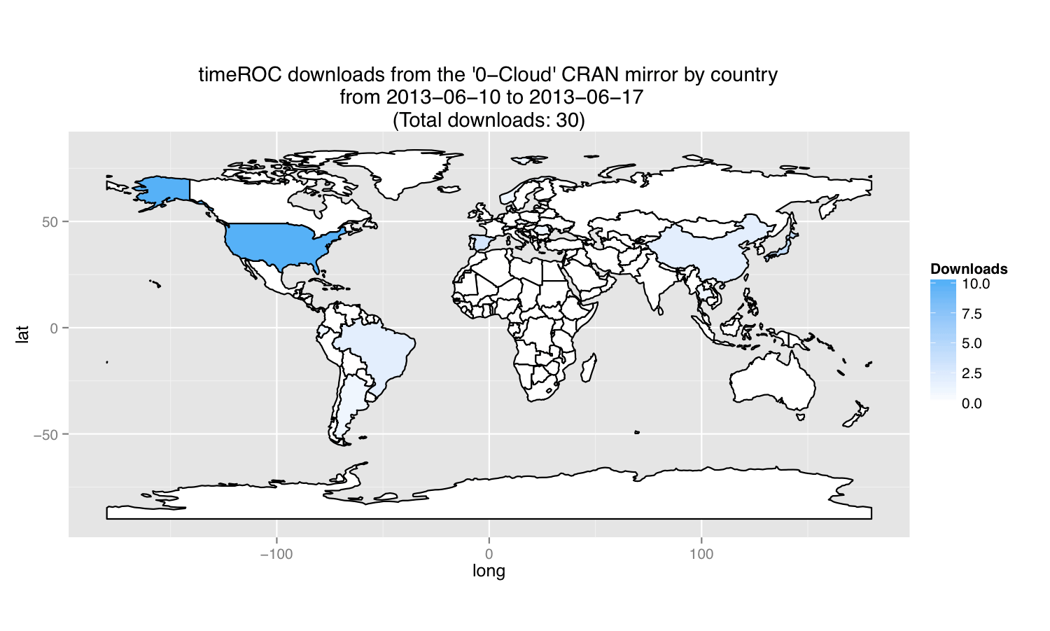
wm <- pkgDNLs.worldmapcolor(pkgname = "timeROC", shp.file.rep = "~/shapefileRepository")
wmHere is an exemple of the result on a friend’s package: timeROC
Update: Thanks to the integration of this function into Tal’s installr package, an easier way to obtain such a map is now to use the following code:
install.packages(devtools)
library(devtools)
install_github("talgalili/installr", username="talgalili")
library(installr)
RStudio_CRAN_data_folder <- download_RStudio_CRAN_data(START = '2013-06-10',
                                                       END = '2013-06-17')
my_RStudio_CRAN_data <- read_RStudio_CRAN_data(RStudio_CRAN_data_folder)
wm <- pkgDNLs_worldmapcolor(pkg_name="timeROC",
                            dataset = my_RStudio_CRAN_data)
wm